Tutorial to use the harmonic Metropolis-Hastings sampling

This tutorial describe how to use the harmonic domain implementation of the method, as described in Leloup et al. 2023.

import os, sys, time
import numpy as np
import healpy as hp
import matplotlib.pyplot as plt
import scipy as sp
import jax
import jax.numpy as jnp
from micmac.third_party import get_instrument, get_observation, get_noise_realization

import micmac

First, define the problem you want to solve

fgs_model = 'd0s0' # Defining the foreground model

# In case you want to use the customized routines, proceeds as follows
# you must then define fgs_model_init for the original model from PySM (here with d7s1 as an example)
# and nside_spv_model for the chosen spatial variatibility of the SEDs
if fgs_model == 'customized_nonparametric' or fgs_model == 'customized_parametric':
    fgs_model_init = ['s1','d7']
    nside_spv_model = 1
    idx_ref_freq = 6 # Index of the reference frequency in the PySM model ; 6 for 93 GHz in the example of LiteBIRD as it corresponds to the 7th frequency channel


noise_seed = 42 # Define the seed for the noise realization
seed_realization_CMB = 43 # Define the seed for the CMB realization

Then, identify the directories for the param files

dir_params = "example_params/"

# The toml file contain the main parameters for the proper initiliazation of the pipeline
param_toml = dir_params + "corr_fullsky_LB_Harmonic.toml"
# The yaml file contain spatial variability parameters which are not relevant here, but are needed for the pipeline to run and essential for the pixel pipeline
param_spv_yaml = dir_params + "params_spv_LB_nside0.yaml"

Afterwards, create the harmonic sampler from the param files

Harm_obj = micmac.create_Harmonic_MICMAC_sampler_from_toml_file(param_toml, param_spv_yaml)

<_io.TextIOWrapper name='example_params/params_spv_LB_nside0.yaml' mode='r' encoding='UTF-8'>
count_b: 26
n_betas:  26

>>> Tree of spv config as passed by the User:
root
  nside_spv
    default: [0]
    f1
      default: None
      b0
        default: None
      b1
        default: None
      b2
        default: None
      b3
        default: None
      b4
        default: None
      b5
        default: None
      b6
        default: None
      b7
        default: None
      b8
        default: None
      b9
        default: None
      b10
        default: None
      b11
        default: None
      b12
        default: None
    f2
      default: [0]
      b0
        default: None
      b1
        default: None
      b2
        default: None
      b3
        default: None
      b4
        default: None
      b5
        default: None
      b6
        default: None
      b7
        default: None
      b8
        default: None
      b9
        default: None
      b10
        default: None
      b11
        default: None
      b12
        default: None

>>> Tree of spv config after filling the missing values:
root
  nside_spv
    default: [0]
    f1
      default: [0]
      b0
        default: [0]
      b1
        default: [0]
      b2
        default: [0]
      b3
        default: [0]
      b4
        default: [0]
      b5
        default: [0]
      b6
        default: [0]
      b7
        default: [0]
      b8
        default: [0]
      b9
        default: [0]
      b10
        default: [0]
      b11
        default: [0]
      b12
        default: [0]
    f2
      default: [0]
      b0
        default: [0]
      b1
        default: [0]
      b2
        default: [0]
      b3
        default: [0]
      b4
        default: [0]
      b5
        default: [0]
      b6
        default: [0]
      b7
        default: [0]
      b8
        default: [0]
      b9
        default: [0]
      b10
        default: [0]
      b11
        default: [0]
      b12
        default: [0]

Note that the object Harm_obj can also be created from MICMAC_Sampler.

Generate input maps

Defining the parameters of the problem using ``fgbuster``

instr_name = Harm_obj.instrument_name

# Define the instrument
if Harm_obj.instrument_name != 'customized_instrument':
    instrument = get_instrument(Harm_obj.instrument_name) # To get the
else:
    with open(path_toml_file) as f:
        dictionary_toml = toml.load(f)
    f.close()
    instrument = micmac.get_instr(Harm_obj.frequency_array, dictionary_toml['depth_p'])

# Get input foreground maps

if fgs_model == 'customized_parametric':
    print(f"Taking customized parametric foreground model {fgs_model_init} downgraded to {nside_spv_model}")
    my_sky, _ = micmac.parametric_sky_customized(
        fgs_model_init,
        Harm_obj.nside,
        nside_spv_model
    )
    freq_maps_fgs_denoised = micmac.get_observation_customized(
        instrument,
        my_sky,
        nside=Harm_obj.nside,
        noise=False
    )[:, 1:, :]   # keep only Q and U
elif fgs_model == 'customized_nonparametric':
    print(f"Taking customized nonparametric foreground model {fgs_model_init} downgraded to {nside_spv_model}")
    freq_maps_fgs_denoised, non_param_fgs_SEDs = micmac.fgs_freq_maps_from_customized_model_nonparam(
        Harm_obj.nside,
        nside_spv_model,
        instrument,
        fgs_models=fgs_model_init,
        idx_ref_freq=idx_ref_freq
        )
elif fgs_model != '':
    print(f"Taking PySM foreground model {fgs_model}")
    freq_maps_fgs_denoised = get_observation(
        instrument,
        fgs_model,
        nside=Harm_obj.nside,
        noise=False
        )[:, 1:, :]  # keep only Q and U
else:
    print("No foreground model specified")
    freq_maps_fgs_denoised = np.zeros((Harm_obj.n_frequencies, Harm_obj.nstokes, Harm_obj.n_pix)) # No foregrounds

Taking PySM foreground model d0s0

OMP: Info #276: omp_set_nested routine deprecated, please use omp_set_max_active_levels instead.

# Get noise maps
np.random.seed(noise_seed)
input_noise_map = get_noise_realization(Harm_obj.nside, instrument)[:, 1:, :]

Assemble everything

freq_maps_fgs = freq_maps_fgs_denoised + input_noise_map

Now retrieving the CMB maps and spectra using the r value given in the params files using CAMB to generate an input CMB spectrum and Healpy to generate the map

np.random.seed(seed_realization_CMB)

input_freq_maps, input_cmb_maps, theoretical_red_cov_r0_total, theoretical_red_cov_r1_tensor = Harm_obj.generate_input_freq_maps_from_fgs(freq_maps_fgs, return_only_freq_maps=False)

Calculating spectra from CAMB !
Calculating spectra from CAMB !

• input_freq_maps contains CMB+foregrounds+noise

• input_cmb_maps only contains CMB (over all frequencies)

• theoretical_red_cov_r0_total is the scalar mode spectrum given with dimensions [lmax+1-lmin, nstokes, nstokes]

• theoretical_red_cov_r1_tensor is the tensor mode spectrum given with dimensions [lmax+1-lmin, nstokes, nstokes]

To recover the classic form of the power specturm [number_correlations,lmax+1-lmin] from the reduced covariance form with dimensions [lmax+1-lmin, nstokes, nstokes], we can call:

theoretical_r0_total = micmac.get_c_ells_from_red_covariance_matrix(theoretical_red_cov_r0_total)
theoretical_r1_tensor = micmac.get_c_ells_from_red_covariance_matrix(theoretical_red_cov_r1_tensor)

The input covariance can be retrieved as:

input_cmb_power_spectrum = theoretical_r0_total + theoretical_r1_tensor * Harm_obj.r_true

Minimally informed approach

In order to do the minimally informed approach described in Leloup et al. 2023, we must define a correction term denoted C_approx.

In the approach, this can correspond to the scalar mode power spectrum, so we can define it as:

c_ell_approx = micmac.get_c_ells_from_red_covariance_matrix(theoretical_red_cov_r0_total)

From here, we have almost all the tools to compute the log-proba associated with the problem, we now need to set up the sampling itself.

First guesses and covariance for the Metropolis-Hastings sampling

We can obtain the B_f covariance and r step-size through Fisher matrices computed prior

ls examples_Fisher_matrices/

Fisher_matrix_LiteBIRD_EB_model_d0s0_noise_True_seed_42_lmin2_lmax128.txt
Fisher_matrix_SO_SAT_EB_model_d0s0_noise_True_seed_42_lmin2_lmax128.txt

dir_Fisher = 'examples_Fisher_matrices/'

inverse_covariance_matrix = np.loadtxt(dir_Fisher + 'Fisher_matrix_LiteBIRD_EB_model_d0s0_noise_True_seed_42_lmin2_lmax128.txt')

covariance_B_f = np.linalg.inv(inverse_covariance_matrix)[:-1, :-1]/100
step_size_r = np.sqrt(np.linalg.inv(inverse_covariance_matrix)[-1, -1])/1

We can compute the exact solutions for \(B_f\) (with d0s0) from a given parametrisation with \(\beta_d\), \(T_d\), \(\beta_s\)

exact_solution_beta_mbb = 1.54
exact_solution_temp_mbb = 20.
exact_solution_beta_pl = -3.

if fgs_model == 'customized_nonparametric':
    init_mixing_matrix_obj = micmac.InitMixingMatrix(
        freqs=Harm_obj.frequency_array,
        ncomp=Harm_obj.n_components,
        pos_special_freqs=Harm_obj.pos_special_freqs,
        spv_nodes_b=Harm_obj.spv_nodes_b,
        non_param_fgs_mixing_matrix=non_param_fgs_SEDs,
        beta_mbb=exact_solution_beta_mbb,
        temp_mbb=exact_solution_temp_mbb,
        beta_pl=exact_solution_beta_pl
    )
    theoretical_params = init_mixing_matrix_obj.init_params()
else:
    init_mixing_matrix_obj = micmac.InitMixingMatrix(
        freqs=Harm_obj.frequency_array,
        ncomp=Harm_obj.n_components,
        pos_special_freqs=Harm_obj.pos_special_freqs,
        spv_nodes_b=Harm_obj.spv_nodes_b,
        beta_mbb=exact_solution_beta_mbb,
        temp_mbb=exact_solution_temp_mbb,
        beta_pl=exact_solution_beta_pl
    )
    theoretical_params = init_mixing_matrix_obj.init_params()

>>> init params built with spectral params: 1.54 20.0 -3.0

And then the first guess:

step_size_B_f = np.diag(sp.linalg.sqrtm(covariance_B_f))

gap_to_true_value = 20

init_params_mixing_matrix = theoretical_params + step_size_B_f * gap_to_true_value * np.random.randn(theoretical_params.size)

As for r, it can be anything sensible (between \(0\) and the current constraint, but not \(0\))

initial_guess_r = 1e-8

The usual approach when considering \(r_{\rm true} = 0\) is to set-up a boundary for the \(r\) sampling, which is done in the following way

# Getting r_min

## We first define the minimum value of r available to keep C(r) positive definite
r_min = -np.min(theoretical_red_cov_r0_total[:,1,1]/theoretical_red_cov_r1_tensor[:,1,1])
Harm_obj.boundary_B_f_r = Harm_obj.boundary_B_f_r.at[0,-1].set(r_min)

We are now fully ready to perform the Harmonic Metropolis-Hastings sampling !

Metropolis-Hastings sampling

As we have loaded from a file the covariance matrix, we can change it by setting the corresponding attribute to Harm_obj

Harm_obj.covariance_B_f = covariance_B_f
Harm_obj.step_size_r = step_size_r

Or we can set it up as the variable covariance_B_f_r to pass to perform_harmonic_MH

covariance_B_f_r = np.zeros((covariance_B_f.shape[0] + 1, covariance_B_f.shape[1] + 1))
covariance_B_f_r[:-1, :-1] = covariance_B_f
covariance_B_f_r[-1, -1] = step_size_r**2

We can change here the number of iterations of the Metropolis-Hastings, otherwise the one by default in the parameter file will be chosen

Harm_obj.number_iterations_sampling = 30000

Then we can run the sampling itself

Harm_obj.perform_harmonic_MH(input_freq_maps,
                             c_ell_approx,
                             init_params_mixing_matrix,
                             initial_guess_r=initial_guess_r,
                             theoretical_r0_total=theoretical_r0_total,
                             theoretical_r1_tensor=theoretical_r1_tensor,
                             covariance_B_f_r=None,
                             print_bool=False)

# Beware: the time displayed on the bar might be wrong and the actual time longer !!

Disabling chex !!!
Starting 30000 iterations for harmonic run

sample: 100%|██████████| 30000/30000 [1:48:30<00:00,  4.61it/s]

End of MH iterations for harmonic run in 108.51840004523595 minutes !

We can then retrieve the chains, which will be in the format [number_iterations+1, size_sample]

all_params_mixing_matrix_samples = Harm_obj.all_params_mixing_matrix_samples
all_r_samples = Harm_obj.all_samples_r

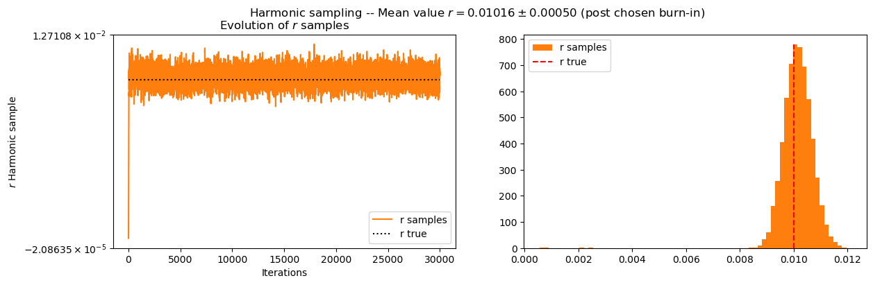
And finally plot the parameters, starting with \(r\):

expected_burn_in = 50 # To be fine-tuned

plt.figure(figsize=(14,4))

# n_sigma = 3

all_r_samples = Harm_obj.all_samples_r

cond = np.arange(Harm_obj.number_iterations_sampling) > expected_burn_in
mean_r = np.round(all_r_samples[cond].mean(), decimals=5)
std_r = np.round(all_r_samples[cond].std(), decimals=5)

alpha_value = .5
color_MICMAC_pixel = 'mediumpurple'
color_MICMAC_pixel_list = ['mediumpurple', 'blue', 'red', 'gold', 'brown']

plt.suptitle("Harmonic sampling -- Mean value $r = {:.5f} \pm {:.5f}$ (post chosen burn-in) ".format(mean_r, std_r))

plt.subplot(121)
plt.plot(np.arange(Harm_obj.number_iterations_sampling), all_r_samples, color='tab:orange', label='r samples')
plt.plot([0, Harm_obj.number_iterations_sampling], [Harm_obj.r_true,Harm_obj.r_true], 'k:', label='r true')


plt.xlabel("Iterations")
plt.ylabel('$r$ Harmonic sample')
plt.title(r'Evolution of $r$ samples')
if Harm_obj.r_true >= 0:
    plt.yscale('symlog')
else:
    plt.yscale('log')
plt.legend()

plt.subplot(122)
hist_values, bins_value, _ = plt.hist(all_r_samples, bins=70, label='r samples', color='tab:orange', density=True)
plt.plot([Harm_obj.r_true,Harm_obj.r_true], [0,hist_values.max()], 'r--', label='r true')
plt.legend()
plt.show()

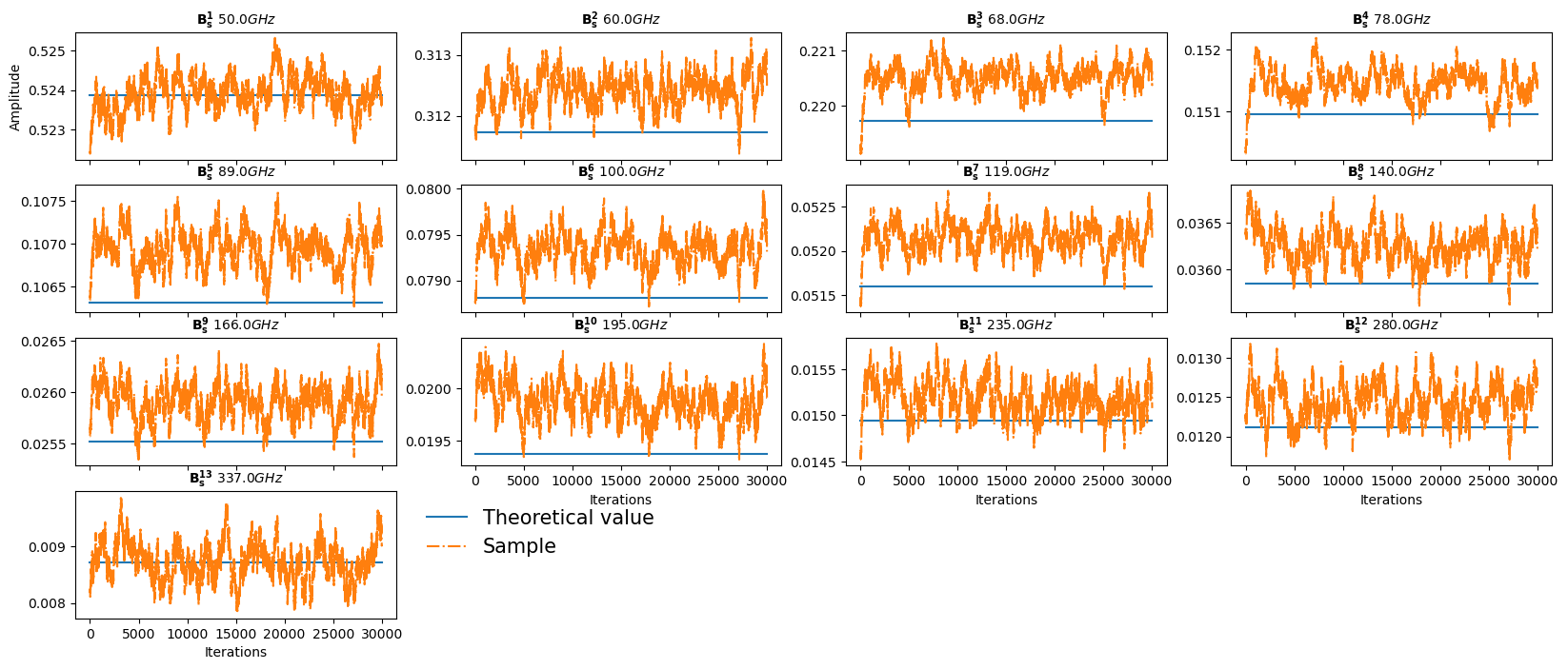
Then \(\bf B_f\)

list_correl = ['EE', 'BB', 'EB']

red_cov_approx_matrix = micmac.get_reduced_matrix_from_c_ell(c_ell_approx)
ell_arange = np.arange(red_cov_approx_matrix.shape[0]) + Harm_obj.lmin

frequency_Bf = np.array(instrument['frequency'][1:-1])
dim_Bf = len(frequency_Bf)
dim_synch = Harm_obj.indexes_b[0,1]
len_pos_special_freqs = len(Harm_obj.pos_special_freqs)


all_B_f_sample_synch = all_params_mixing_matrix_samples[:,:dim_synch]
all_B_f_sample_dust = all_params_mixing_matrix_samples[:,dim_synch:]

frequency_array = np.array(instrument['frequency'])

n_columns = 4
number_rows = (Harm_obj.n_frequencies-len_pos_special_freqs)//n_columns + 1

fontsize_titles = 10
fontsize_label = 10

fig, ax = plt.subplots(number_rows, n_columns, figsize=(20,8))
useless_plots = number_rows*n_columns - (Harm_obj.n_frequencies-len_pos_special_freqs)
for idx_useless in range(0,useless_plots):
    num_row = (number_rows*n_columns)//n_columns
    num_col = (number_rows*n_columns)%n_columns
    fig.delaxes(ax[num_row-1, num_col-idx_useless-1])

# fig.suptitle(f"Mixing matrix first component parameters sampled vs iterations", fontsize=14)

for i in range(Harm_obj.n_frequencies-len_pos_special_freqs):
    num_row = i//n_columns
    num_col = i%n_columns
    # ax[num_row, num_col].set_title((f'Synch ${frequency_Bf[i]} GHz$'))
    ax[num_row, num_col].set_title('$\mathbf{B_s^{'+f'{i+1}'+'}\ }$' + f'${frequency_Bf[i]} GHz$', fontsize=fontsize_titles, fontdict=dict(weight='bold'))

    ax[num_row, num_col].plot([0,Harm_obj.number_iterations_sampling+1], [theoretical_params[i],theoretical_params[i]], label='Theoretical value')
    ax[num_row, num_col].plot(np.arange(Harm_obj.number_iterations_sampling), all_B_f_sample_synch[:,i], '-.', label='Sample')

    cond = np.where(np.arange(Harm_obj.number_iterations_sampling+1) > expected_burn_in)[0]
    mean_B_f = np.round(all_B_f_sample_synch[cond,i][cond].mean(), decimals=5)
    std_B_f = np.round(all_B_f_sample_synch[cond,i][cond].std(), decimals=5)

    mean_value = all_B_f_sample_synch[:,i].mean()
    # ax[num_row, num_col].plot([0,Harm_obj.number_iterations_sampling+1], [mean_B_f,mean_B_f], ':', label='Samples mean post burn-in')

    if i == 0:
        ax[num_row, num_col].set_ylabel('Amplitude', fontsize=fontsize_label)
    if i >= Harm_obj.n_frequencies-len_pos_special_freqs-n_columns:
        ax[num_row, num_col].set_xlabel('Iterations', fontsize=fontsize_label)
    else:
        ax[num_row, num_col].tick_params(axis='x', labelbottom=False)
ax[num_row, num_col].legend(bbox_to_anchor=(1.04, 1), loc="upper left", prop={'size': 15}, frameon=False)

fig, ax = plt.subplots(number_rows, n_columns, figsize=(20,8))
useless_plots = number_rows*n_columns - (Harm_obj.n_frequencies-len_pos_special_freqs)
for idx_useless in range(0,useless_plots):
    num_row = (number_rows*n_columns)//n_columns
    num_col = (number_rows*n_columns)%n_columns
    fig.delaxes(ax[num_row-1, num_col-idx_useless-1])

# fig.suptitle(f"Mixing matrix second component parameters sampled vs iterations", fontsize=14)
for i in range(Harm_obj.n_frequencies-len_pos_special_freqs):
    num_row = i//n_columns
    num_col = i%n_columns
    # ax[num_row, num_col].set_title((f'Dust ${frequency_Bf[i]} GHz$'))
    ax[num_row, num_col].set_title('$\mathbf{B_d^{'+f'{i+1}'+'}\ }$' + f'${frequency_Bf[i]} GHz$', fontsize=fontsize_titles, fontdict=dict(weight='bold'))

    ax[num_row, num_col].plot([0,Harm_obj.number_iterations_sampling+1], [theoretical_params[i+dim_synch],theoretical_params[i+dim_synch]], label='Theoretical value')
    ax[num_row, num_col].plot(np.arange(Harm_obj.number_iterations_sampling), all_B_f_sample_dust[:,i], '-.', label='Sample')

    cond = np.where(np.arange(Harm_obj.number_iterations_sampling+1) > expected_burn_in)[0]
    mean_B_f = np.round(all_B_f_sample_dust[cond,i].mean(), decimals=5)
    std_B_f = np.round(all_B_f_sample_dust[cond,i].std(), decimals=5)

    mean_value = all_B_f_sample_dust[:,i].mean()
    # ax[num_row, num_col].plot([0,Harm_obj.number_iterations_sampling+1], [mean_B_f,mean_B_f], ':', label='Samples mean post burn-in')
    if i == 0:
        ax[num_row, num_col].set_ylabel('Amplitude', fontsize=fontsize_label)
    if i >= Harm_obj.n_frequencies-len_pos_special_freqs-n_columns:
        ax[num_row, num_col].set_xlabel('Iterations', fontsize=fontsize_label)
    else:
        ax[num_row, num_col].tick_params(axis='x', labelbottom=False)
ax[num_row, num_col].legend(bbox_to_anchor=(1.04, 1), loc="upper left", prop={'size': 15}, frameon=False)
plt.show()

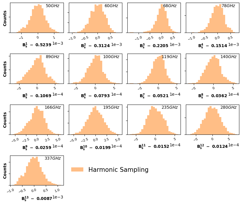
And the corresponding histograms, a good test to check if the distribution is Gaussian or not

burn_in = -30000 # To be fine-tuned

bins_number = 25

list_correl = ['EE', 'BB', 'EB']

frequency_Bf = np.array(Harm_obj.frequency_array[1:-1])
dimension_free_param_B_f = 2*(Harm_obj.n_frequencies-len_pos_special_freqs)
dim_freq_B_f = len(frequency_Bf)

alpha_value = .5
Harm_color = ['tab:orange']

fontsize_titles = 10
fontsize_label = 10

mean_Harm_synch = Harm_obj.all_params_mixing_matrix_samples[burn_in:,:dim_freq_B_f].mean(axis=0)
mean_Harm_dust = Harm_obj.all_params_mixing_matrix_samples[burn_in:,dim_freq_B_f:].mean(axis=0)

all_B_f_sample_synch = Harm_obj.all_params_mixing_matrix_samples[burn_in:,:dim_freq_B_f] - mean_Harm_synch
all_B_f_sample_dust = Harm_obj.all_params_mixing_matrix_samples[burn_in:,dim_freq_B_f:] - mean_Harm_dust


frequency_array = np.array(Harm_obj.frequency_array)

if Harm_obj.n_frequencies-len_pos_special_freqs >= 10:
    number_columns = 4
    number_rows = (Harm_obj.n_frequencies-len_pos_special_freqs)//number_columns + 1

    fig, ax = plt.subplots(number_rows, number_columns, figsize=(10,8))
    plt.subplots_adjust(hspace=.7, wspace=.1)
    useless_plots = number_rows*number_columns - (Harm_obj.n_frequencies-len_pos_special_freqs)
    for idx_useless in range(0,useless_plots):
        num_row = (number_rows*number_columns)//number_columns
        num_col = (number_rows*number_columns)%number_columns
        fig.delaxes(ax[num_row-1, num_col-idx_useless-1])

    for i in range(Harm_obj.n_frequencies-len_pos_special_freqs):
        num_row = i//number_columns
        num_col = i%number_columns
        ax[num_row, num_col].text(.8, .9, f'${frequency_Bf[i]} GHz$',
                                horizontalalignment='center',
                                verticalalignment='center',
                                fontsize=fontsize_titles,
                                transform=ax[num_row, num_col].transAxes)
        ax[num_row, num_col].xaxis.set_tick_params(labelsize=8)
        ax[num_row, num_col].ticklabel_format(style='sci', axis='both', scilimits=(0,0))
        plt.setp(ax[num_row, num_col].get_xticklabels(), rotation=20, horizontalalignment='center')

        hist_values, bins_value, _ = ax[num_row, num_col].hist(all_B_f_sample_synch[:,i], bins=bins_number, density=True, color=Harm_color[0], alpha=alpha_value, label='Harmonic Sampling')

        if num_col == 0:
            ax[num_row, num_col].set_ylabel('Counts', fontsize=fontsize_label, fontdict=dict(weight='bold'))
        ax[num_row, num_col].tick_params(axis='y', labelleft=False)

        ax[num_row, num_col].set_xlabel('$\mathbf{B_s^{'+f'{i+1}'+'}\ -}$'+' {:.4f}'.format(mean_Harm_synch[i]), fontsize=fontsize_label, fontdict=dict(weight='bold'))
    ax[num_row, num_col].legend(bbox_to_anchor=(1.04, 0.8), loc="upper left", prop={'size': 15}, frameon=False)
    # plt.loglog()

    fig, ax = plt.subplots(number_rows, number_columns, figsize=(10,8))
    plt.subplots_adjust(hspace=.7, wspace=.1)
    useless_plots = number_rows*number_columns - (Harm_obj.n_frequencies-len_pos_special_freqs)
    for idx_useless in range(0,useless_plots):
        num_row = (number_rows*number_columns)//number_columns
        num_col = (number_rows*number_columns)%number_columns
        fig.delaxes(ax[num_row-1, num_col-idx_useless-1])

    for i in range(Harm_obj.n_frequencies-len_pos_special_freqs):
        num_row = i//number_columns
        num_col = i%number_columns
        ax[num_row, num_col].text(.8, .9, f'${frequency_Bf[i]} GHz$',
                                horizontalalignment='center',
                                verticalalignment='center',
                                fontsize=fontsize_titles,
                                transform=ax[num_row, num_col].transAxes)
        ax[num_row, num_col].xaxis.set_tick_params(labelsize=8)
        ax[num_row, num_col].ticklabel_format(style='sci', axis='both', scilimits=(0,0))
        plt.setp(ax[num_row, num_col].get_xticklabels(), rotation=20, horizontalalignment='center')

        hist_values, bins_value, _ = ax[num_row, num_col].hist(all_B_f_sample_dust[:,i], bins=bins_number, density=True, color=Harm_color[0], alpha=alpha_value, label='Harmonic Sampling')

        if num_col == 0:
            ax[num_row, num_col].set_ylabel('Counts', fontsize=fontsize_label, fontdict=dict(weight='bold'))
        ax[num_row, num_col].tick_params(axis='y', labelleft=False)

        ax[num_row, num_col].set_xlabel('$\mathbf{B_d^{'+f'{i+1}'+'}\ -} $'+' {:.4f}'.format(mean_Harm_dust[i]), fontsize=fontsize_label, fontweight='bold')

    ax[num_row, num_col].legend(bbox_to_anchor=(1.04, 0.8), loc="upper left", prop={'size': 15}, frameon=False)
    # plt.loglog()

plt.show()

The final values will be given by the average of the chains

last_samples_to_take = 10000 # Last samples to take for the mean and std computation -- To fine-tune

# Getting <B_f>
final_B_f = all_params_mixing_matrix_samples[-last_samples_to_take:,:].mean(axis=0)

# Getting <r>
final_r = all_r_samples[-last_samples_to_take:].mean()

Then we can plot the corresponding residuals

c_ell_true_CMB = micmac.get_c_ells_from_red_covariance_matrix_JAX(theoretical_red_cov_r0_total + Harm_obj.r_true*theoretical_red_cov_r1_tensor)
c_ell_CMB_r2 = micmac.get_c_ells_from_red_covariance_matrix_JAX(theoretical_red_cov_r0_total + 0.01*theoretical_red_cov_r1_tensor)
c_ell_lensing = micmac.get_c_ells_from_red_covariance_matrix_JAX(theoretical_red_cov_r0_total)

mean_params_list = [final_B_f]
method_name = ['Harmonic']

# Residuals power spectrum


colorstyle_list = ['tab:orange','tab:blue','tab:green','tab:red','tab:purple','tab:brown','tab:pink','tab:gray','tab:olive','tab:cyan']

indices_polar = np.array([1,2,4])

linewidth_plots = 3

fig, axes = plt.subplots(figsize=(14,8))

ell_array = np.arange(Harm_obj.lmin, Harm_obj.lmax+1)

# Plotting as D_ell = ell*(ell+1)/(2*pi) C_ell
factor_ell = (ell_array*(ell_array+1))/(2*np.pi)

# Plotting the CMB power spectra for reference
plt.plot(ell_array, c_ell_true_CMB[1,:]*factor_ell, color='red', linewidth=linewidth_plots, label='input BB')
plt.plot(ell_array, c_ell_CMB_r2[1,:]*factor_ell, 'k-.', linewidth=linewidth_plots, label='BB primordial (r=0.01)')
plt.plot(ell_array, c_ell_lensing[1,:]*factor_ell, color='darkgray', linewidth=linewidth_plots, label='lensing BB')


# Getting N
freq_inverse_noise = micmac.get_noise_covar_extended(np.array(instrument['depth_p']), Harm_obj.nside)

# Getting the residuals
for i in range(len(mean_params_list)):
    mean_mixing_matrix = Harm_obj.get_B_from_params(mean_params_list[i])
    recovered_CMB_Wd_mean = micmac.get_Wd(freq_inverse_noise,
                                            mean_mixing_matrix,
                                            (input_freq_maps-input_cmb_maps-input_noise_map),
                                            jax_use=False)[0, :, :]
    print("Values pixel res fgs: mean", np.abs(recovered_CMB_Wd_mean).mean(), "std", np.abs(recovered_CMB_Wd_mean).std(), "max", np.abs(recovered_CMB_Wd_mean).max())

    recovered_res_wo_CMB_mean = micmac.get_Wd(freq_inverse_noise,
                                                mean_mixing_matrix,
                                                input_freq_maps,
                                                jax_use=False)[0, :, :] - input_cmb_maps[0]
    recovered_CMB_Wd_mean_extended = np.vstack([np.zeros_like(recovered_CMB_Wd_mean[0]), recovered_CMB_Wd_mean])
    c_ells_recovered_CMB_Wd_mean = hp.anafast(recovered_CMB_Wd_mean_extended, lmax=Harm_obj.lmax, iter=Harm_obj.n_iter)[2,Harm_obj.lmin:]#/f_sky
    recovered_res_wo_CMB_mean_extended = np.vstack([np.zeros_like(recovered_res_wo_CMB_mean[0]), recovered_res_wo_CMB_mean])
    c_ells_recovered_res_wo_CMB_mean = hp.anafast(recovered_res_wo_CMB_mean_extended, lmax=Harm_obj.lmax, iter=Harm_obj.n_iter)[2,Harm_obj.lmin:]#/f_sky

    ell_array = np.arange(c_ells_recovered_CMB_Wd_mean.shape[-1])+Harm_obj.lmin

    factor_ell = (ell_array*(ell_array+1))/(2*np.pi)


    label_Stat_res = f"{method_name[i]} Total Residuals"
    label_Syst_res = f'{method_name[i]} Foreground Residuals'

    linestyle_dashdotted = '-.'

    plt.plot(ell_array,
                c_ells_recovered_res_wo_CMB_mean*factor_ell,
                linestyle=linestyle_dashdotted,
                linewidth=linewidth_plots,
                color=colorstyle_list[i],
                label=label_Stat_res, alpha=.8)

    linestyle_dotted = ':'

    plt.plot(ell_array,
                c_ells_recovered_CMB_Wd_mean*factor_ell,
                linestyle=linestyle_dotted,
                linewidth=linewidth_plots,
                color=colorstyle_list[i],
                label=label_Syst_res, alpha=.8)

if Harm_obj.instrument_name == 'LiteBIRD':
    plt.loglog()
else:
    plt.yscale('log')

plt.ylabel("$D^{BB}_\ell$ [$uK^2$]",fontsize=18)
plt.xlabel(r"$\ell$",fontsize=18)
plt.tick_params(axis='both', which='major', labelsize=12)
plt.tick_params(axis='both', which='minor', labelsize=12)

# Cosmetic putting "Satellite" in the top left corner
plt.text(.1, .95, 'Satellite',
                        horizontalalignment='center',
                        verticalalignment='center',
                        fontsize=18,
                        transform=axes.transAxes)

plt.legend(bbox_to_anchor=(1.25, .7), loc='upper center', prop={'size': 18}, frameon=False)
plt.show()

Values pixel res fgs: mean 0.001388342728361142 std 0.002159539144143462 max 0.05277580593007514